Blog-- Thoughts on data analysis, software development and innovation management. Comments are welcome Post 64 Natural Language Processing: forthcoming online classes at Stanford, and a unified approach with Multilayer Neural Networks22-Jan-2012Needless to say, I was very eager to begin the nlp-class tomorrow. It's a pity that it has just been delayed for administrative reasons. But good things take time, so we'd better be patient 'cos this looks very good (45000 people expecting its launch, this is incredibly exciting). Having used Manning's and Jurafsky's masterpieces for years, it is now enthralling to have the chance to attend their classes, getting my hands dirty with the classical problems, techniques and the whole lot of details of statistical NLP. But with time one gets to become a little agnostic with respect to the idealisation of some method for solving a particular problem. Let me elaborate on this. For instance, given a classification problem and a particular complexity for a discriminating function, does it really matter to learn the boundary with a Maximum Entropy principle (e.g., Logistic Regression), or with a Maximum Margin criterion (e.g., Support Vector Machine)? Will the optimised functions be much different? Assuming that the two classifiers are successfully trained (i.e., they are pertinently regularised, so no overfitting problems exist, and they are still complex enough for the problem at hand, so no underfitting either), my experience tells me that the particular learning philosophy/scheme (MaxEnt vs. Max-Margin) is reduced to a minimum. And this feeling (also supported by evidence) is shared with other researchers such as Alexander Osherenko (see our public discussion on the Corpora-List), and Ronan Collobert, who even developed a fully unified approach based on Multilayer Neural Networks (MNN) as the universal learners (*) to tackle a variety of typical NLP tasks, including Part-Of-Speech tagging, chunking, Named Entity Recognition and Semantic Role Labelling. In his own words: "it is often difficult to figure out which ideas are most responsible for the state-of-the-art performance of a large ensemble (of classifiers)". In this regard, in (Collobert, et al., 2011), see Remark 4 (Conditional Random Fields), it is also specifically noted how other techniques such as CRFs have been applied to the same NLP tasks with similar results. So there are plenty of choices to attain the same goals and the interest (IMO) comes down to discussing the one that could best fit in the situation/problem. To me this is synonymous with contributing to knowledge, although MNNs are generally regarded as black boxes that lack human interpretation. In fact, this is the seed of a critical discussion (Collobert, et al., 2011). (*) The proposed generic neural network discovers useful features in large unlabelled datasets, which enable it to perform close to the state-of-the-art. This approach is presented in contrast to relying on a priori knowledge (e.g., domain heuristics). Task-specific engineering (i.e., that does not generalise to other tasks) is not desirable in this multiple task setting (Collobert, et al., 2011).
-- Post 63 L-systems, fractal plants and grammars24-Dec-2011One beautiful example of life is vegetation. In fact, since I was little I had always believed that ferns were supposed to be the first form of life on Earth, but now I see that the Wikipedia debunks this fact here. Anyhow, plants do deserve a lot of admiration and respect, they are fascinating to me. I myself grow a vegetable garden (especially for cultivating tomatoes with the seeds that my grandfather carefully selected for over 40 years), I annually visit the St. Boi and Molins expositions of agriculture and farming, and I own two exemplars of John Seymour's books on horticulture. However, since I am also a computer enthusiast, seeing such beauty in the form of an algorithm is a doubly rewarding experience to me. In this regard, I here release my implementation of an L-system (see the CODE section). L-systems are a mathematical formalism originally aimed at modelling the growth processes of plant development. The basic idea is to define complex objects by successively replacing parts of a simple object using a set of rewriting rules, aka productions. These production rules can be carried out recursively and in parallel (in contrast to Chomsky grammars, which are applied sequentially). The biological motivation of L-systems is to interpret a character string as a sequence of drawing instructions. Here is where turtle graphics come in handy, otherwise the generated object would be very difficult to describe by standard Euclidean geometry. The Logo programming language is one example of such turtle graphics system. See what can be generated with the fractal plant and tree definitions that L-system provides:
 The linguistic motivation of L-systems lies in the grammar that defines them. The former examples were produced with deterministic grammars, which means that there is exactly one production rule for each symbol in the grammar's alphabet. However, this implementation of L-system also allows defining multiple rules per symbol, i.e., a stochastic grammar, and the choice is made according to an uniform distribution among the available choices. If this concept takes a textual form, the pair of sentences:
may be produced with a single L-system with the following definition:
The source code organisation of L-system follows common FLOSS directives (such as src folder, doc, README, HACKING, COPYING, etc.). It only depends externally on the Boost Iostreams Library for tokenising the definition file, and it makes use of the premake build script generation tool. Additionally, a Logo code interpreter is needed to graphically represent the production. I hope you enjoy it. By the way, Merry Xmas! Post 62 Principal Component Analysis for Blind Source Separation? Shouldn't you use Independent Component Analysis instead?02-Dec-2011This week's work in the Machine Learning class has treated the Principal Component Analysis (PCA) procedure to reduce the dimensionality of the feature space. The use of the Singular Value Decomposition (SVD) of the covariance matrix of the features has reminded me of the introductory video to unsupervised learning where Prof. Ng applies the SVD to blindly separate speech sound sources (e.g., the cocktail party problem). And I have felt puzzled because as far as I know, the problem of Blind Source Separation (BSS) boils down to finding a linear representation in which the components are statistically independent, uncorrelatedness is not enough (Hyvarinen, et al., 2001). Independence is a much stronger property than uncorrelatedness. Considering the BSS problem, many different uncorrelated representations of the signals that would not be independent and would not separate the sources could be found. Uncorrelatedness in itself is not enough to separate the components. This is also the reason why PCA (or factor analysis) cannot separate the signals: they give components that are uncorrelated, but little more. In this regard, Independent Component Analysis (ICA) finds underlying factors or components from multivariate (multidimensional) statistical data that are both statistically independent and nongaussian. Nongaussianity is a fundamental requirement that also explains the main difference between ICA and PCA, in which the nongaussianity of the data is not taken into account (for gaussian data, uncorrelated components are always independent). In fact, ICA could be considered as nongaussian factor analysis. In reality, the data often does not follow a gaussian distribution, and the situation is not as simple as PCA assumes. For example, many real-world signals have supergaussian distributions, e.g., the speech signal follows a Laplacian distribution (Gazor and Zhang, 2003). This means that the random variables, i.e., the signals, take relatively more often values that are very close to zero or very large. Seeing Prof. Ng solving the BSS problem with PCA does indeed surprise me, but I certainly doubt that the solution may be happily explained with a single Matlab/Octave one-liner. I have myself done some experimentation (for the sake of empirical evidence) with the noise cancellation scenario that is suggested in my signal processing class, and I can definitely state that PCA cannot separate voice from noise. In actual fact, both the speech signal and the noise signal differ considerably from the Gaussian distributions that are assumed in PCA, see (Gazor and Zhang, 2003) and the figure below, respectively.
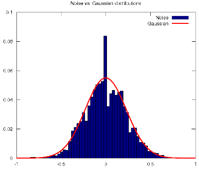 The noise used to produce the histogram in the figure corresponds to the rotor of a helicopter.
-- Post 61 Support Vector Machines and the importance of regularisation to approach the optimal boundary27-Nov-2011In this post I would like to show some empirical evidence about the importance of model regularisation in order to control the complexity so as to not overfit the data and generalise better. To this end, I make use of this week's work on Support Vector Machines (SVM) in the Machine Learning class. Firstly, a scenario similar to Post 52 is settled. Then, the optimal Bayes boundary is drawn, along with an unregularised SVM (C=100). Up to this point, the performance of this classifier is expected to be as modest as the former unregularised Logistic Regression: since it is tightly dependent on the observed samples, the slope of the linear boundary differs a lot from the optimum. Instead, when a considerable amount of regularisation is applied, i.e., a SVM with C=1, the model is more conservative and reticent to classify outliers, so its final slope approaches the optimum, thus increasing its expected effectiveness.
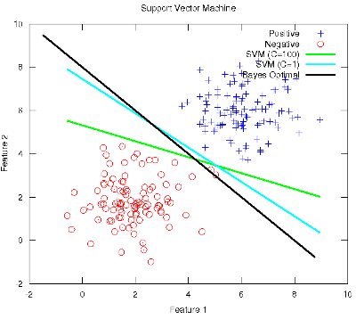 The Octave code used to generate the figure is available here. Note that the rest of the ml-class files need to be present along with the former. Post 60 On figuring out the similarity between the Mean Squared Error and the Negative Corpus LogLikelihood in the cost function for optimising Multilayer Neural Networks23-Nov-2011This long post title links with my previous Post 59, where I discussed using different criteria for the cost function and for the derivation of the gradient when training Multilayer Neural Networks (MNN) with Backpropagation. After a fruitful chat with Prof. Xavier Vilasis and some careful reading (Bishop, 2006) and (Hastie, et al., 2003), I have eventually come to realise there is no mystery, as long as the right assumptions are made. The gist of the discussion is the error of the trained model wrt the data, along with its form and/or its distribution. Bishop (2006) shows that this error function can be motivated as the maximum likelihood solution under an assumed Gaussian noise model. Note that the normal distribution has maximum entropy among all real-valued distributions with specified mean and standard deviation. By applying some calculus, the negative log of a Gaussian yields a squared term, which determines the form of the cost function, just as the Mean Squared Error (MSE). Hence, the two optimisation criteria converge to a similar quadratic form, and this explains their freedom to interchange. Although not all real-life problems are suitable for such Gaussian noise model, e.g., the quantisation error has an approximately uniform distribution, the normal distribution of the error is plausibly assumed for the majority of situations. What follows is some experimentation considering 1) the impact of the nature of the data and 2) the fitting of the model to attain this Gaussian noise model. In this regard, (1) is evaluated by classifying data from a well-defined Gaussian distribution and (first) from a pure random distribution (generated by radioactive decay), and (second) from its "equivalent" Gaussian model (by computing the mean and the variance of the points in the random sample). Given that two Gaussians with the same variance are to be discriminated in the end, the optimal Bayes boundary is a line perpendicular to the segment that links their means, passing through its mid-point, see Post 52. Therefore, the MNN model does not need to be very complex. This is accomplished with one hidden layer with two units, and (2) is evaluated by applying different levels of regularisation (this design is ensured not to underfit the data). If the assumption for Gaussian noise model holds, the error should be normally distributed and the effectiveness rates for the MSE and the Neg Corpus LogLikelihood costs should be similar. Without regularisation
With regularisation
Given the results, it is observed how the actual nature of the data has a little impact on the analysis as the effectiveness trends (measured with the Accuracy rate in the table) are similar for both scenarios in all settings. The determining factor so as to assume a normally distributed error, which embraces the Gaussian noise model, is the fitting of the model wrt the data. This leads to allowing some regularisation. When the model overfits the data (i.e., without regularisation), its poor generalisation yields a varied range of error samples that distances from the normal distribution, hence the different effectiveness rates between MSE and Neg LogLikelihood costs. Instead, when the model fits the data well (i.e., with regularisation, resulting in a complex-enough model that can generalise well), the range of error samples is more narrow (i.e., the error samples are more comparable) and its distribution approaches the Gaussian form, hence the similar effectiveness rates between MSE and Neg LogLikelihood costs. Note that only in this maximum entropy model setting, the classifier contains the maximum amount of (Fisher) information from the data, so this is the optimum model (i.e., optimum parameter values) for a given network structure. The code used to conduct the experiments is available here.
-- Post 59 Different cost criteria in Multilayer Neural Network training19-Nov-2011It is customary to train Multilayer Neural Networks (MNN) with the Mean Squared Error (MSE) criterion for the cost function (Duda, et al., 2001), especially when the Backpropagation algorithm is used, which is presented as a natural extension of the Least Mean Square algorithm for linear systems, a deal of lexical coincidences with "mean square" altogether. Nevertheless, Prof. Ng in the ml-class presented a somewhat different flavour of cost function for training MNN, recurring to the "un-log-likelihood" error, i.e., the negative of the corpus loglikelihood, that typically characterises the Logistic Regression error wrt the data, and for a good reason:
Not only is the Neg. Corpus LogLikelihood a more effective cost function than the traditional MSE, it is also twice faster to train using Backpropagation with a MNN, at least for the digits recognition task. Check out the cost function code here. In addition, it shows that the advanced optimisation method does its job regardless of the underlying matching criteria between the cost function and the gradients. That's awesome.
-- Post 58 Inter-language evaluation of sentiment analysis with granular semantic term expansion17-Nov-2011Yesterday, my Master Student Isaac Lozano defended his thesis with honours. The topic of his work entitles this post: inter-language evaluation of sentiment analysis with granular semantic term expansion. His work is mainly framed by our former publication (Trilla et al., 2010), but he has extended it by porting EmoLib to Spanish in its entirety and evaluating its performance wrt English, which is the default working language, and also the most supported one by the research community. His contribution principally consists in improving the Word-Sense Disambiguation module in order to profit from the knowledge contained in the Spanish WordNet ontology, to then expand the term feature space with the synsets of the observed words with their correct senses. To accomplish this goal, a Lucene index of WordNet needs to be created first, along with the Information-Content-based measures that help determine the semantic similarity/relatedness among the terms (e.g., with Conrath-Jiang, Resnik, etc), a la JavaSimLib. In fact, to perform a more granular analysis, several WordNet indices need to be created, one for each word-class with a possible amount of affect, i.e., content words such as nouns, verbs and adjectives. This granularity wrt the Part-Of-Speech is assumed to be of help to increase the identification of affect in text, see (Pang and Lee, 2008). Nevertheless, he concluded his work by showing that such intuitive considerations do not deliver a clear improvement in any of the two languages, at least for the datasets at hand: the Semeval 2007 and the Advertising Database. However, he pointed out several interesting ideas regarding the flaws he observed during the development of his work, such as the consideration of lemmas instead of stems in order to increase the retrieval rate from WordNet, or the consideration of antonyms instead of synonyms in case negations are observed in the text of analysis. Allow me to express my congratulations. Now that EmoLib performs in Spanish as well as in English, the new language version of the demo service has just been made available here. Enjoy.
-- Post 57 Spanish Government presidential candidates face-off analytics15-Nov-2011This post is in line with a recent article that presents a novel application to signal the polarity of opinions in Twitter posts, see this piece of news published by Universidad de Alicante. The original work is centred on the face-off debate between Rajoy and Rubalcaba, the two main candidates for the Spanish Government presidential election that will take place next Sunday. I here reproduce a similar experiment with the default configuration of EmoLib, which is grounded on a centroid-based classifier representing the words' emotional dimensions in the circumplex, but with the transcription of the whole debate, which is available for the two candidates: Rajoy, on behalf of the PP, and Rubalcaba, on behalf of the PSOE. What follows is a table that shows some linguistic statistics regarding their speeches (bearing in mind that they spoke the same amount of time):
In contrast to the original article where only positive and negative tags were provided, EmoLib allows a more granular analysis with the additional "neutral" label, which lies in between the opposing extreme positive and negative labels. According to the statistics, note that both candidates have a similar speaking style. Perhaps Rubalcaba is more prone to expose his ideas incrementally while Rajoy prefers to put them forward at once, since the former has articulated 15 paragraphs more than the latter in the same amount of time. Anyhow, the richness of the vocabulary employed is similar (taken for the rate between the size of the vocabulary and the total amount of spoken words). Maybe what is most surprising is that the affective figures delivered by this study end up being contrary to the original ones, since Rajoy spoke positively 32.99% of the time while Rubalcaba did it a 35.71%. The rates continue being more of less comparable, but the trend is inverted wrt what has been originally published. Post 56 Multi-class Logistic Regression in Machine Learning (revisited)10-Nov-2011In my former post about Multi-class Logistic Regression in ML (see Post 55), I questioned the ml-class about using a multi-class generalisation strategy, i.e., the One-Versus-All (OVA), with a plain dichotomic Logistic Regression classifier when there's a more concise multi-class model, i.e., the Multinomial Logistic Regression (MLR), that is already of extensive use in ML. I foolishly concluded (to err is human) that using OVA should be due to higher effectiveness issues, assuming that my MLR optimisation implementation based on batch Gradient Descent was directly comparable to the one provided in class, which is based on an advanced optimisation procedure, "with steroids", such as Conjugate Gradient or L-BFGS. Specifically, the course provides a method based on the Polack-Ribiere gradient search technique, which uses first and second order derivatives to determine the search direction, and the Wolfe-Powell conditions, which lead to fast minimisation of the criterion function, altogether suited for efficiently dealing with a large number of parameters. But as Prof. Ng remarked in a previous lecture, the optimisation procedure has a notable impact on the final fitting of the model wrt the training data, and this definitely makes the difference. I have recoded the MLR with the parameter unrolling method shown this week in order to interface with the same advanced optimisation method (available here), so the results are now truly directly comparable. The MLR yields an effectiveness of 95.22% in 99.58 seconds, which makes it 0.2% more effective and 10.91 times faster than OVA-LR. Therefore, the class-wise parameter dependence in the MLR predictions provides an overall much faster to train and slightly better classifier than OVA-LR, for this problem. Nevertheless, the question wrt which strategy is preferable still remains open because other multi-class strategies such as Pairwise classification are yet to be studied. Post 55 Multi-class Logistic Regression in Machine Learning06-Nov-2011This week's assignment of the ml-class deals with multi-class classification with Logistic Regression (LR) and Neural Networks. In this post I would like to focus on the former method, though, in line with Post 52. There I missed the use of the Multinomial LR (MLR) to tackle multi-class problems, putting in question the need of a multi-category generalisation strategy, i.e., One-Versus-All (OVA), when there is already a model that inherently integrates this multi-class issue, i.e., MLR. Now, after conducting some experimentation (see the table below), I shall conclude that it must be due to its higher effectiveness, which is measured wrt the accuracy rate, at least for the proposed digit-recognition problem.
Both these methods learn some discriminant functions and assign a test instance to the category corresponding to the largest discriminant (Duda, et al., 2001). Specifically, the OVA-LR learns as many discriminant functions as the number of classes, but the MLR learns one function less because it firstly sets the parameters for one class (the null vector) and then learns the rest in concordance with this setting without loss of generality (Carpenter, 2008). Therefore, the essential difference is that OVA-LR learns the discriminants independently, while MLR needs all class-wise discriminants for each prediction, so they cannot be trained independently. This dependence characteristic may then flaw the final system effectiveness a little (in fact, it only makes 3% worse), but in contrast, it learns at a much faster rate (8.43 times faster given this data).
The code that implements the MLR, which is available
here
(it substitutes "oneVsAll.m" in "mlclass-ex3"),
is based on (Carpenter, 2008). Nevertheless, a
batch version has been produced in order to avoid the imprecision
introduced by the online approximation,
see Post 51,
Actually, this MLR is not directly comparable to the OVA-LR developed in class because it is optimised with a different strategy. A fair comparison regarding this optimisation aspect is conducted and explained in the following post, see Post 56
-- newer | older - RSS - Search |
|||||||||||||||||||||||||||||||||||||||||||||||||||||||||||||||||||||||||||||||||||||||||||
All contents © Alexandre Trilla 2008-2025 |