Blog-- Thoughts on data analysis, software development and innovation management. Comments are welcome Post 62 Principal Component Analysis for Blind Source Separation? Shouldn't you use Independent Component Analysis instead?02-Dec-2011This week's work in the Machine Learning class has treated the Principal Component Analysis (PCA) procedure to reduce the dimensionality of the feature space. The use of the Singular Value Decomposition (SVD) of the covariance matrix of the features has reminded me of the introductory video to unsupervised learning where Prof. Ng applies the SVD to blindly separate speech sound sources (e.g., the cocktail party problem). And I have felt puzzled because as far as I know, the problem of Blind Source Separation (BSS) boils down to finding a linear representation in which the components are statistically independent, uncorrelatedness is not enough (Hyvarinen, et al., 2001). Independence is a much stronger property than uncorrelatedness. Considering the BSS problem, many different uncorrelated representations of the signals that would not be independent and would not separate the sources could be found. Uncorrelatedness in itself is not enough to separate the components. This is also the reason why PCA (or factor analysis) cannot separate the signals: they give components that are uncorrelated, but little more. In this regard, Independent Component Analysis (ICA) finds underlying factors or components from multivariate (multidimensional) statistical data that are both statistically independent and nongaussian. Nongaussianity is a fundamental requirement that also explains the main difference between ICA and PCA, in which the nongaussianity of the data is not taken into account (for gaussian data, uncorrelated components are always independent). In fact, ICA could be considered as nongaussian factor analysis. In reality, the data often does not follow a gaussian distribution, and the situation is not as simple as PCA assumes. For example, many real-world signals have supergaussian distributions, e.g., the speech signal follows a Laplacian distribution (Gazor and Zhang, 2003). This means that the random variables, i.e., the signals, take relatively more often values that are very close to zero or very large. Seeing Prof. Ng solving the BSS problem with PCA does indeed surprise me, but I certainly doubt that the solution may be happily explained with a single Matlab/Octave one-liner. I have myself done some experimentation (for the sake of empirical evidence) with the noise cancellation scenario that is suggested in my signal processing class, and I can definitely state that PCA cannot separate voice from noise. In actual fact, both the speech signal and the noise signal differ considerably from the Gaussian distributions that are assumed in PCA, see (Gazor and Zhang, 2003) and the figure below, respectively.
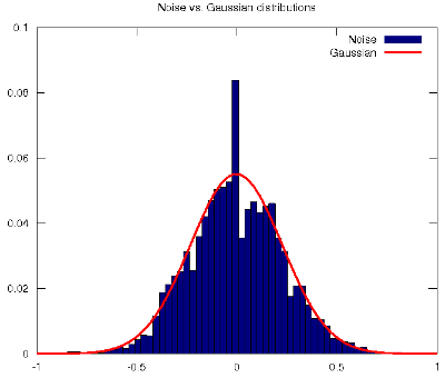 The noise used to produce the histogram in the figure corresponds to the rotor of a helicopter.
-- |
All contents © Alexandre Trilla 2008-2025 |